 ScoreSync News
Open App
ScoreSync News
Open App
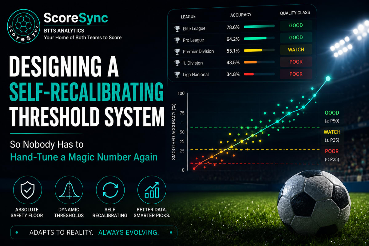
Designing a Self-Recalibrating Threshold System — So Nobody Has to Hand-Tune a Magic Number Again
A few weeks ago, I was reviewing a Sunday slate of automated football predictions when one result immediately looked wrong.
Sitting at #2 in our Match Result category was:
Hødd vs Strømmen — Norway 1. divisjon
The fixture itself carried a model confidence score of 92%. On the surface, that looked strong. But the historical reliability behind the league told a very different story:
- Results reliability: 43.5%
- Team Strength reliability: 54.5%
Neither number was particularly convincing.
On a three-way market such as Home/Draw/Away, a purely random baseline is roughly one-third. So 43.5% is only modestly above chance, while 54.5% is better but still nowhere near the level I would expect from a league appearing near the top of a curated “best picks” list.
Yet the fixture had outranked many alternatives from leagues with much stronger historical performance.
That was the clue that something deeper was wrong.
The bug wasn’t confidence. It was what we meant by “reliable”
Tracing the selection pipeline back through the code revealed a surprisingly simple problem.
The system had only one meaningful eligibility axis:
How much history do we have for this league?
If a league had enough settled predictions, it became a high-evidence league. In our terminology, that meant Level A.
The problem was that Level A said nothing about whether those settled predictions had actually been good.
A league with 50 settled predictions at 80% accuracy and another with 50 settled predictions at 35% accuracy were both structurally treated as mature, trustworthy candidates.
The system knew that both leagues had a lot of evidence.
It did not distinguish between:
a lot of evidence that the model works
and
a lot of evidence that the model performs badly.
That distinction matters.
In fact, the second case should make us less willing to trust a league, not more.
The ranking logic then compounded the problem. Once the league passed the sample-size gate, fixture-level confidence could dominate the ranking. A single 92-confidence prediction could pull a mediocre league near the top, even when the historical reliability table was warning us not to trust it.
The fix was not simply to “add an accuracy check.”
The real challenge was designing an accuracy system that would still make sense six months later.
⸻
The obvious fix — and why it is wrong
The first instinct is something like this:
if (league.smoothedAccuracy < 55) {
return null;
}
It looks reasonable.
It is also wrong.
The problem is that 55% accuracy does not mean the same thing in every prediction market.
For a three-way Match Result market, where the possible outcomes are Home, Draw and Away, a 55% hit rate can represent a meaningful edge.
For a binary market such as BTTS Yes/No, where a naïve baseline is much closer to 50%, 55% may be only marginally better than noise.
For Over 1.5 goals, the situation changes again. This is structurally an easier market in many leagues. A healthy model may routinely produce league-level accuracy in the high 70s or low 80s. A 55% hit rate there would not be “acceptable.” It would be a warning sign.
So one global threshold creates two problems at once:
- it is too strict for some markets;
- it is dangerously lenient for others.
There is also a second problem that is easier to miss.
A threshold such as 55% is usually chosen from whatever the model looked like on the day somebody typed that number into the source code.
But models change.
Data grows.
Leagues behave differently over time.
Prediction quality improves, deteriorates, or becomes more stable.
A fixed threshold slowly stops representing what it originally meant.
A threshold that never adapts becomes a fossil.
⸻
The solution: separate evidence from quality
The first architectural change was to stop treating sample size and prediction quality as the same concept.
We now classify each league-market combination along two independent axes.
Evidence level
This answers:
How much history do we have?
For example:
- A — strong sample
- B — moderate sample
- C — limited evidence
This part already existed and remains useful.
Quality class
This answers:
How good has the model actually been?
The new classes are:
- GOOD
- WATCH
- POOR
That means a league can now be:
- A / GOOD
- A / WATCH
- A / POOR
- B / GOOD
- B / WATCH
- B / POOR
and so on.
This distinction immediately changes the meaning of a league with a large sample but poor accuracy.
An A / POOR league is not a mature league we should trust.
It is a league where we have strong evidence that the model is performing badly.
That league should be excluded.
⸻
The second challenge: how do you define GOOD without creating another magic number?
This is where the system became more interesting.
The classification uses two layers:
GOOD =
smoothedAccuracy >= Math.max(
absoluteGoodFloor,
dynamicGoodThreshold
);
WATCH =
smoothedAccuracy >= Math.max(
absoluteWatchFloor,
dynamicWatchThreshold
);
POOR = neither;
Each layer solves a different problem.
⸻
Layer 1: the absolute floor
The absolute floor is a permanent, market-specific safety net.
Its job is not to define what “good” means forever.
Its job is to prevent a weak population from grading itself generously.
For example:
export const QUALITY_THRESHOLD_DEFAULTS = {
RESULT_WIN: {
absoluteGoodFloor: 58,
absoluteWatchFloor: 48
},
BTTS_YES: {
absoluteGoodFloor: 62,
absoluteWatchFloor: 52
},
BTTS_NO: {
absoluteGoodFloor: 62,
absoluteWatchFloor: 52
},
OU_2_5: {
absoluteGoodFloor: 65,
absoluteWatchFloor: 52
},
OU_1_5: {
absoluteGoodFloor: 75,
absoluteWatchFloor: 65
}
};
These are deliberately different.
Match Result has a lower natural baseline than BTTS.
Over 1.5 has a higher floor than Over 2.5 because reliable Over 1.5 leagues tend to cluster at much stronger hit rates.
The floor is therefore market-aware.
But importantly, the floor is only a minimum standard.
It is not the entire threshold.
⸻
Layer 2: the dynamic threshold
The dynamic threshold is the part that prevents the system from going stale.
Every time picks are generated, the system takes the current population of league reliability scores for that market and calculates fresh percentile boundaries.
A simple percentile helper looks like this:
export function computePercentile(sortedAscValues, p) {
const n = sortedAscValues.length;
if (n === 0) return null;
if (n === 1) return sortedAscValues[0];
const rank = (p / 100) * (n - 1);
const lowIdx = Math.floor(rank);
const highIdx = Math.ceil(rank);
if (lowIdx === highIdx) {
return sortedAscValues[lowIdx];
}
const fraction = rank - lowIdx;
return sortedAscValues[lowIdx] +
fraction *
(sortedAscValues[highIdx] - sortedAscValues[lowIdx]);
}
Before selecting picks, we build the current qualified population:
const populationAccuracies = computed
.filter(c =>
c.evidenceSampleSize >= thresholds.levelBSampleMin &&
c.smoothedAccuracy != null
)
.map(c => c.smoothedAccuracy)
.sort((a, b) => a - b);
Then calculate:
const dynamicGoodThreshold =
computePercentile(populationAccuracies, 50);
const dynamicWatchThreshold =
computePercentile(populationAccuracies, 25);
In plain English:
GOOD means being at least as strong as the current median of comparable leagues, while still clearing the absolute safety floor.
WATCH uses the lower percentile boundary, again subject to its own absolute floor.
That means the definition of good performance naturally moves with the system.
If the model improves across the whole league population, the threshold rises.
If the market matures and performance spreads out, the bar adjusts.
Nobody needs to notice that the old constant has become outdated.
Nobody needs to open the code and change 55 to 58.
The system recalibrates itself.
⸻
Why both layers are necessary
Either approach on its own has a serious weakness.
Dynamic threshold without an absolute floor
Imagine a new prediction market where every league is performing badly.
If the median is only 43%, then half of the leagues would technically sit above the median.
Without a floor, the system might call some of them GOOD simply because they are less bad than their peers.
That is not good enough.
Absolute floor without a dynamic layer
This solves the first problem but recreates the fossil.
If the model improves significantly over time and nearly every league clears the same old floor, the threshold stops discriminating between genuinely excellent leagues and merely acceptable ones.
The combination solves both problems:
Absolute floor → prevents a race to the bottom
Dynamic threshold → prevents the rule becoming stale
Using Math.max() means both conditions matter.
⸻
The population-size guard rail
There is another statistical trap.
A percentile calculated from two or three leagues is not very meaningful.
Early in a market’s life, there may not be enough mature leagues to calculate a stable population-relative threshold.
So we added a minimum population size:
export const MIN_POPULATION_FOR_DYNAMIC_THRESHOLD = 5;
If fewer than five leagues have enough evidence to participate in the population:
- the dynamic percentile layer is disabled;
- classification falls back to the absolute market floor.
The system therefore avoids pretending it has a statistically meaningful population distribution when it does not.
This is an important design principle:
when the data is insufficient, simplify the model rather than fabricate precision.
⸻
The most important property: nothing is permanently labelled GOOD or POOR
This is what makes the system genuinely self-recalibrating.
There is no permanent database record saying:
Norway 1. divisjon = WATCH
MLS = GOOD
Ykkönen = POOR
There is also no administrator-maintained list deciding which leagues are trustworthy.
The classification is recomputed from the latest settled performance every time picks are generated.
The loop becomes:
Prediction
→ Result settles
→ Reliability updates
→ League quality is recalculated
→ Future picks use the new classification
A league can therefore move naturally:
GOOD → WATCH → POOR
or recover:
POOR → WATCH → GOOD
without a code change, deployment or manual intervention.
That matters because model performance is not static.
A competition that was difficult for the model three months ago may become predictable as more data accumulates.
Another may deteriorate.
The system should respond to what the evidence says now.
⸻
Testing time, not just state
One of the most useful tests for this system was not a traditional “input → output” test.
It tested behaviour over time.
test(
'a league automatically reclassifies as new results settle',
async () => {
// Phase 1:
// 20 settled predictions, all wrong.
await seedHistory({
correct: 0,
wrong: 20
});
await computeLeagueReliabilityProfiles(
db,
asOfDate1
);
assert.equal(
profileAt(asOfDate1).quality_class,
'POOR'
);
// Phase 2:
// Another 40 predictions settle correctly.
await seedHistory({
correct: 40,
wrong: 0
});
await computeLeagueReliabilityProfiles(
db,
asOfDate2
);
assert.equal(
profileAt(asOfDate2).quality_class,
'GOOD'
);
}
);
No configuration changed.
No source code changed.
No admin toggled anything.
Only the evidence changed.
The classification followed it.
That is the behaviour we wanted.
⸻
One thing we deliberately do freeze
There is an important distinction between:
today’s live classification of a league
and
the classification that justified a historical pick.
The first should always be dynamic.
The second should never change.
When a pick is generated, we snapshot the evidence that supported that decision:
ALTER TABLE daily_top_picks
ADD COLUMN IF NOT EXISTS evidence_level TEXT;
ALTER TABLE daily_top_picks
ADD COLUMN IF NOT EXISTS quality_class TEXT;
A production implementation can also retain:
- reliability source;
- raw accuracy;
- smoothed accuracy;
- sample size;
- threshold values;
- final selection score;
- generation timestamp.
Suppose a league was classified GOOD when a pick was generated on Tuesday.
Three weeks later, its performance deteriorates and it becomes WATCH.
The live system should use WATCH for new predictions.
But the Tuesday pick must continue to say:
this fixture was selected when the league was GOOD under the threshold population that existed at that time.
That is not stale data.
It is an audit trail.
The difference is important.
We do not store:
“this league is permanently GOOD.”
We store:
“this decision was made using a GOOD classification at this point in time.”
That makes historical analysis reproducible.
⸻
What changed for the fixture that started the investigation
Once the new quality dimension was introduced, the original examples behaved very differently.
Hødd vs Strømmen
Historical evidence:
- Results reliability: 43.5%
- Team Strength reliability: 54.5%
- high fixture confidence
Old system:
Large sample
→ Level A
→ fully eligible
→ raw confidence dominates
→ ranked #2
New system:
Large sample
→ Level A evidence
→ WATCH quality
→ secondary candidate only
Its high confidence can no longer allow it to outrank genuinely GOOD league candidates.
A more extreme case
Another selected league had approximately:
- Results reliability: 34.8%
- Team Strength reliability: 21.7%
Under the old system, enough settled history meant it could still qualify as Level A.
Under the new system:
Evidence = A
Quality = POOR
and POOR is a hard exclusion.
The fixture’s own confidence is never even considered.
That ordering is intentional.
Reliability controls whether the fixture deserves consideration.
Fixture confidence controls where an eligible fixture ranks.
Those are different jobs.
⸻
Match Result needed one extra rule
Our Match Result model has two independent historical reliability signals:
- Results accuracy
- Team Strength accuracy
Different leagues respond differently to each.
Some are better predicted through the normal Result model.
Others respond much more strongly to team-strength differences.
So the system can resolve a league to:
RESULTS
TEAM_STRENGTH
COMBINED
But there is a subtle distinction here too.
The question:
Which signal is stronger?
is not the same as:
Is the stronger signal actually trustworthy?
Suppose:
Results = 34.8%
Team Strength = 21.7%
RESULTS is the stronger signal.
But 34.8% is still poor.
So source resolution happens first, and quality classification happens second.
The same principle applies to COMBINED.
Two mediocre signals should not become “strong” simply because they agree.
COMBINED is reserved for cases where both sources independently provide meaningful positive evidence.
⸻
The broader lesson
This started as a football prediction problem, but the architecture applies much more widely.
Any system that ranks or classifies items from a changing population eventually runs into the same questions:
- Is this score actually good?
- Good compared with what?
- How much evidence supports it?
- What happens when the population improves?
- What happens when the population deteriorates?
- Can a static threshold still mean the same thing six months later?
The mistake is to answer all of those questions with one hardcoded number.
The more robust pattern is:
Evidence quantity
+
Absolute safety floor
+
Population-relative threshold
+
Continuous recalculation
+
Historical decision snapshots
The absolute floor defines the minimum level of sanity.
The population-relative threshold defines what strong performance means right now.
Continuous recalculation allows classifications to evolve as the data evolves.
Historical snapshots preserve explainability without freezing the live model.
The result is not a system with better magic numbers.
It is a system designed so that magic numbers matter less in the first place.